johnkemeny.com

My blogoverse buddy (B_vB^TM) Jonathan asked me to contribute to CoM-18, which he is hosting and I am happy to do so. But first a belated shoutout to my B_vB, and best reviewer, Dave Marain, who interviews Professor Lynn Steen, a principal architect of the original NCTM Standards and a highly respected voice in reform mathematics.

Don’t expect any research topics here. This is about solving a practical problem in automotive gas economy which involves a pricing anomoly, a Greek mathmatician who may have tutored Alexander the Great, and an 18th century Scottish math professor who almost loses his job by taking an unauthorized 2-year sabbatical to tour the Continent. Can you imagine not losing your job today?

So what is the problem? I have 2 cars, an older model which uses regular gas, and a slightly newer model which only uses the more expensive high-test gas, but also gets more miles per gallon (mpg). The question is which is more economical to  drive? The pricing anomaly I have observed is that no matter the price per gallon (ppg) of gasoline, and the price has fluctuated up and down quite a bit, the difference in price between regular and high-test is almost always a constant, viz., 25 cents. So which car  is more economical to drive actually depends on the price of gasoline! Observe.

The price per mile, ppm = price per gallon / miles per gallon.  The percent difference in ppm between regular and high-test,

%diff = (ppm_regular / ppm_high-test) – 1 = (p / m) – 1,

where p = ppg_regular / ppg_high-test and

m = mpg_regular / mpg_high-test.

If we take

d = ppg_high-test – ppg_regular = $0.25 and

m = 25 / 27 and

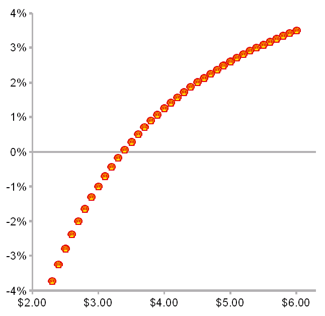
then plot ppg_high-test against %diff we get:

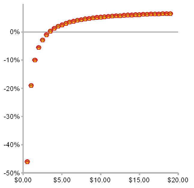
So if the price of high-test is below about $3.35 the gas guzzler is more economical fuel-wise, and versa vice. But what is this  curve? A cubic polynomial trend line fits it almost perfectly. So is it a polynomial? Zooming out gives us a clue.

It is a rectangular hyperbola (first studied by Menaechmus, a student of Plato, about 350 BC) flipped on the X axis and asymptotic to X = 0 and Y = 0.08 = (1 / m) -1. You can easily see this by rewriting the equation for %diff as

%diff = A / ppg_high-test + B where

A = -d / m and

B = (1 / m) – 1

So this leaves the question of why a cubic polynomial fits the data so well. And here is where our Scottish math professor, Colin MacLaurin, comes in. In 1742 he wrote A Treatise on Fluxions (pdf), the first systematic application  of Newton’s calculus, in which he shows, among other trigonometric marvels, how the equation for a hyperbola could be closely approximated by truncating an infinite polynomial series.

This entry was posted on Thursday, October 4th, 2007 at 3:36 am and is filed under Books, Math & Science, Travel. You can follow any responses to this entry through the RSS 2.0 feed. Both comments and pings are currently closed.